How To Do Residual Plot On Ti 84

Regression modeling is the process of finding a office that approximates the relationship between the two variables in 2 information lists. The table shows the types of regression models the TI-84 Plus calculator can compute.

Types of Regression Models

TI-Command	Model Type	Equation
Med-Med	Median-median	y = ax + b
LinReg(ax+b)	Linear	y = ax + b
QuadReg	Quadratic	y = ax2 + bx + c
CubicReg	Cubic	y = ax3 + bx2 + cx + d
QuartReg	Quartic	y = ax4 + bx3 + cx2 + dx + e
LinReg(a+bx)	Linear	y = a + bx
LnReg	Logarithmic	y = a + b*ln(x)
ExpReg	Exponential	y = abx
PwrReg	Ability	y = axb
Logistic	Logistic	y = c/(1 + a*e-bx)
SinReg	Sinusoidal	y = a*sin(bx + c) + d

To compute a regression model for your two-variable data, follow these steps:

1. If necessary, plow on Diagnostics and put your calculator in Part mode.

   When Stat Diagnostics is turned on, the estimator displays the correlation coefficient (r) and the coefficient of determination (r² or R² ) for appropriate regression models (as shown in the tertiary screen). By default, Stat Diagnostics is turned off.

   If the regression model is a function that you want to graph, you must first put your calculator in Function mode.

   Hither's how to plough Stat Diagnostics on and set your calculator to Function fashion:

   1. Press [Fashion].

   2. Use the pointer keys to highlight STAT DIAGNOSTICS ON and printing [ENTER].

   3. Utilize the arrow keys to highlight Office and printing [ENTER].

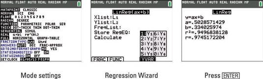
      The first screen shows this procedure.

      

2. Select a regression model from the Stat Calculate menu to activate the Regression Wizard.

   To access the Stat Calculate carte du jour, printing

   

   Repeatedly press the down-pointer key until the number or letter of the desired regression model is highlighted, and printing [ENTER] to select that model.

3. Enter the name for the Xlist data and enter the name of the Ylist data.

4. If necessary, enter the name of the frequency listing.

5. With your cursor in the Store RegEQ line, enter the proper noun of the function (Y₁, ... , Y_nine, or Y₀) in which the regression model is to be stored.

   To enter a function proper noun, press a$ to access the shortcut Y-VAR menu and and so enter the number of the function you want, as shown in the second screen.

6. Press [ENTER] on CALCULATE to view the equation of the regression model.

   This is illustrated in the third screen. The equation of the regression model is automatically stored in the Y= editor nether the name y'all entered in Footstep 5.

Graphing a regression model

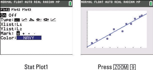
Oft, it is a good idea to take a wait at the scatter plot of your data to determine what blazon of regression model is all-time. Here are the steps to graph a scatter plot of your data and the regression model on the same graph:

1. If you haven't already done and then, graph your two-variable data in a scatter plot or an xy-line plot.

   Gear up up the besprinkle plot past pressing [2nd][Y=][ENTER]. Run into Stat Plot1 in the starting time screen.

   

2. Press [ZOOM][9] to see the graph of your information and regression model.

   This procedure is illustrated in the second screen.

Virtually This Article

About the book writer:

Jeff McCalla is a mathematics teacher at St. Mary'due south Episcopal School in Memphis, TN. He cofounded the TI-Nspire SuperUser group, and received the Presidential Award for Excellence in Science & Mathematics Teaching.

C.C. Edwards is an educator who has presented numerous workshops on using TI calculators.

This article can be found in the category:

• Graphing Calculators ,

Source: https://www.dummies.com/article/technology/electronics/graphing-calculators/regression-modeling-on-the-ti-84-plus-160903/

Share this post